pacman::p_load(readxl)
pacman::p_load(readr)
pacman::p_load(ggstatsplot)
pacman::p_load(ggbraid)
pacman::p_load(gganimate)
pacman::p_load(transformr , gifski)
pacman::p_load(dplyr , lubridate )
pacman::p_load(tidyverse)Take Home Exercise 04
The Task
In this take-home exercise, we need to uncover the impact of COVID-19 as well as the global economic and political dynamic in 2022 on Singapore bi-lateral trade (i.e. Import, Export and Trade Balance) by using appropriate analytical visualisation techniques learned in Lesson 6: It’s About Time.
Background information is that Singapore is a small country with no natural resources. However on the other hands, as robust trade hub and a strong economy, Singapore maintains a relatively stable and strong currency SGD, which gives her a strong advantage for Singapore import as strong Singapore SGD can be used to purchase more goods and services from other countries.
Throughout 2020, 2021 and 2022, Singapore (and the world) just exited the severe climates of Covid pandemics, lockdown lead to disruption of manufacturing, and physical trades, which affect the supply of many commodities / consumer goods. It is a popular belief that as 2022 rolled around, Singapore will be able to leverage on its strong SGD to improve its trade balance.
Let’s examine the data and dive deeper into Singapore trade volumes.
The Data
For the purpose of this take-home exercise, Merchandise Trade provided by Department of Statistics, Singapore (DOS) will be used. The data are available under the sub-section of Merchandise Trade by Region/Market. The study period should be between January 2020 to December 2022.
I) IMPORT VERSUS EXPORT
We want to do a comparison between Singapore Import and Export, first let’s import the data.
monthlyexport_overall <- read_excel("C:/thomashoanghuy/ISSS608-VAA/TakehomeEx/data3/outputFile.xlsx", sheet = "T1")

monthlyimport_overall <- read_excel("C:/thomashoanghuy/ISSS608-VAA/TakehomeEx/data3/outputFile.xlsx", sheet = "T8")
Please note all these figures are in Singapore dollar currency.
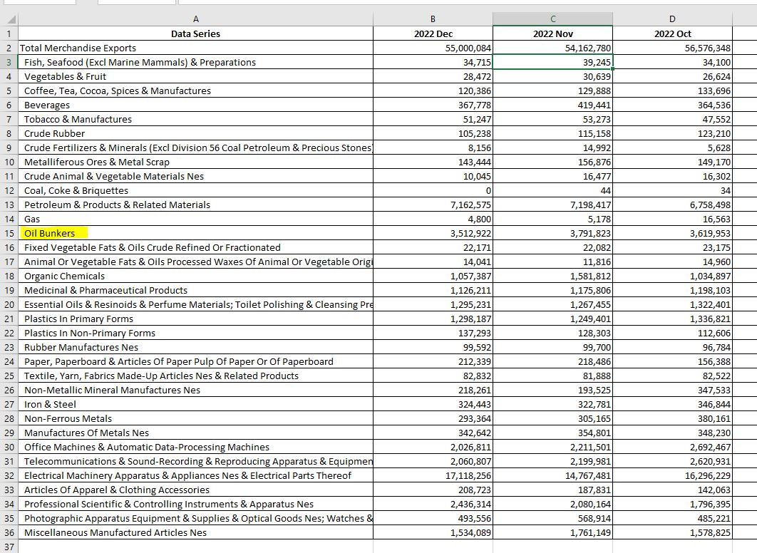
Sheet T1 = Merchandise Exports By Commodity Division, Monthly snippet
Sheet T2 = Merchandise Imports By Commodity Division, Monthly snippet
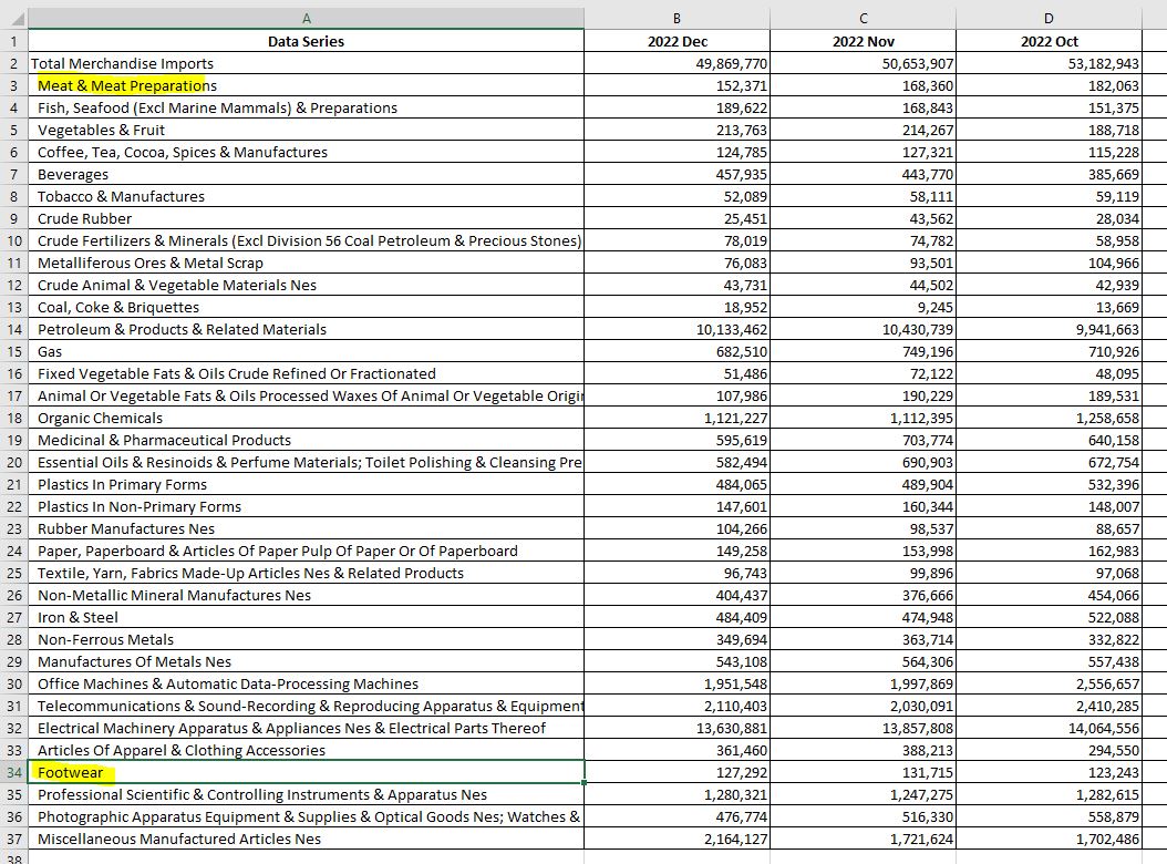
As you can see from above 2 snippets of the data table, most of the sub categories are similar between export and import data. However the highlight rows are some of the differences between the 2 sets of data. We should remove them before we can start any comparisons.
monthlyexport_overall <- monthlyexport_overall[!grepl("Oil Bunkers", monthlyexport_overall$`Data Series`),]monthlyimport_overall <- monthlyimport_overall[!grepl("Meat & Meat Preparations", monthlyimport_overall$`Data Series`),]
monthlyimport_overall <- monthlyimport_overall[!grepl("Footwear", monthlyimport_overall$`Data Series`),]Now both tables would have the same sub categories of merchandises for comparison.
Now. we can extract the total Export Merchandise Import and Export and we can combine them into a separate dataframe
monthlyexport_total <- monthlyexport_overall[grepl("Total Merchandise Exports", monthlyexport_overall$`Data Series`),]monthlyimport_total <- monthlyimport_overall[grepl("Total Merchandise Imports", monthlyimport_overall$`Data Series`),]monthly_tradebalance1 = rbind(monthlyexport_total , monthlyimport_total)
monthly_tradebalance1= as.data.frame(t(monthly_tradebalance1))
colnames(monthly_tradebalance1) <- monthly_tradebalance1[1,]
monthly_tradebalance1 <- monthly_tradebalance1[-1,]
head(monthly_tradebalance1) Total Merchandise Exports Total Merchandise Imports
2022 Dec 55000084 49869770
2022 Nov 54162780 50653907
2022 Oct 56576348 53182943
2022 Sep 62507132 55799312
2022 Aug 63363749 58466009
2022 Jul 64124991 61029374monthly_tradebalance <- monthly_tradebalance1 %>%
rownames_to_column(var = "Month-Year")Reverse sort the data frame “monthly_tradebalance”
monthly_tradebalance <- monthly_tradebalance[nrow(monthly_tradebalance):1, ]
rownames(monthly_tradebalance) <- rownames(monthly_tradebalance[nrow(monthly_tradebalance):1, ])

head(monthly_tradebalance)
Month-Year Total Merchandise Exports Total Merchandise Imports
1 2020 Jan 44501656 41180224
2 2020 Feb 43512320 39472637
3 2020 Mar 45800019 40433029
4 2020 Apr 39946596 35878828
5 2020 May 36482259 31458238
6 2020 Jun 40640766 35120892Convert Month-Year into time format (continuous time series)
monthly_tradebalance$`Month-Year` <- as.Date(paste0(monthly_tradebalance$`Month-Year`, " 01"), format = "%Y %b %d")Convert trade volumes numbers from string to numeric values.
monthly_tradebalance$`Total Merchandise Exports` <- as.numeric(monthly_tradebalance$`Total Merchandise Exports`)
monthly_tradebalance$`Total Merchandise Imports` <- as.numeric(monthly_tradebalance$`Total Merchandise Imports`)
monthly_tradebalanceMelt <- reshape2::melt(monthly_tradebalance, id.var='Month-Year')p1 = ggplot(monthly_tradebalanceMelt, aes(x=monthly_tradebalanceMelt$`Month-Year` , y=value, col=variable, group = 1)) +
geom_point() + geom_line(aes(group=factor(variable))) +
xlab("Year") + ylab("Trade Volume in Billions")
p1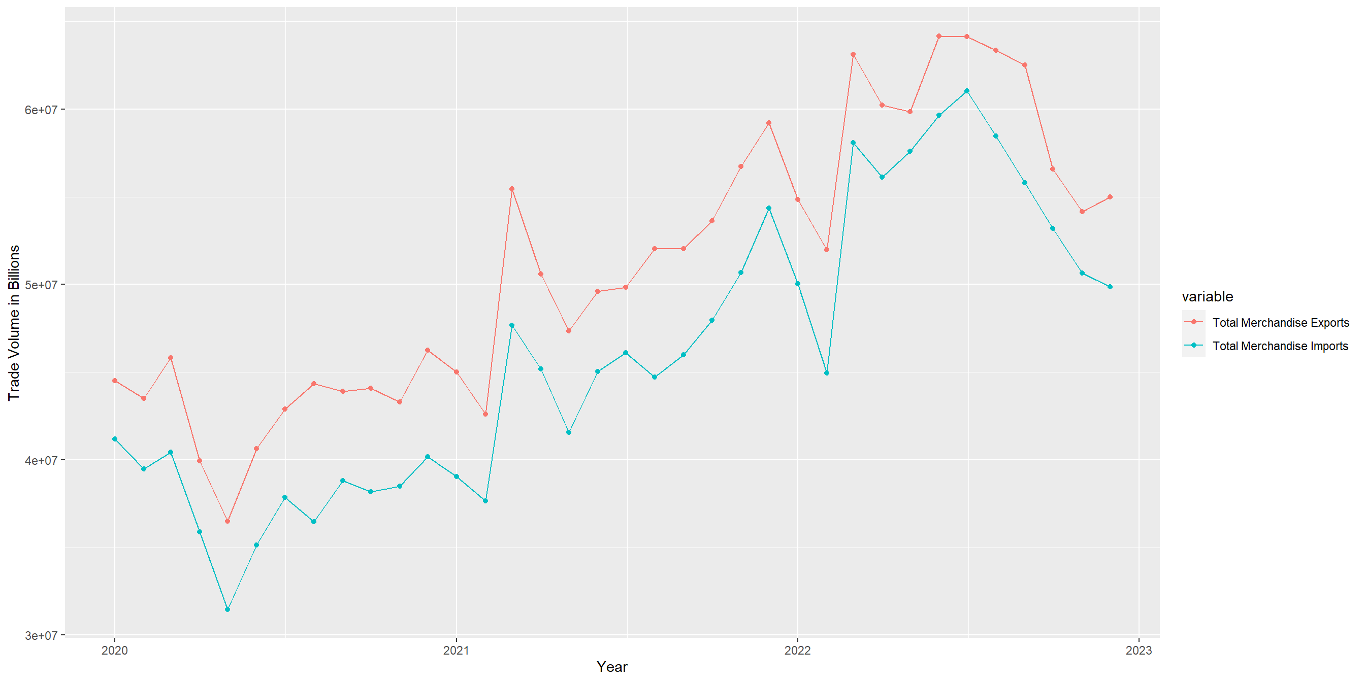
As evidenced by the above chart, Singapore import and export move quite in tandem with each other. Between 2020-2023, it shows an uptrend. As Export volume increase, so does Import. However Singapore overall Export are more than its Import, consistently since post-covid 2020, Singapore is sill a country with a positive trade surplus overall.
While positive trade surplus are confirmed, we should examine how Singapore trade surplus is trending post-covid, let’s create a data table of the difference between Export and Import ( the trade surplus)
monthly_tradebalance$Trade_surplus = monthly_tradebalance$`Total Merchandise Exports` - monthly_tradebalance$`Total Merchandise Imports`p2<- ggplot(monthly_tradebalance, aes(x=monthly_tradebalance$`Month-Year` , y= monthly_tradebalance$Trade_surplus, group = 1)) +
geom_point() + geom_line() + geom_smooth()+
xlab("Year") + ylab("Trade Surplus in Billions")
p2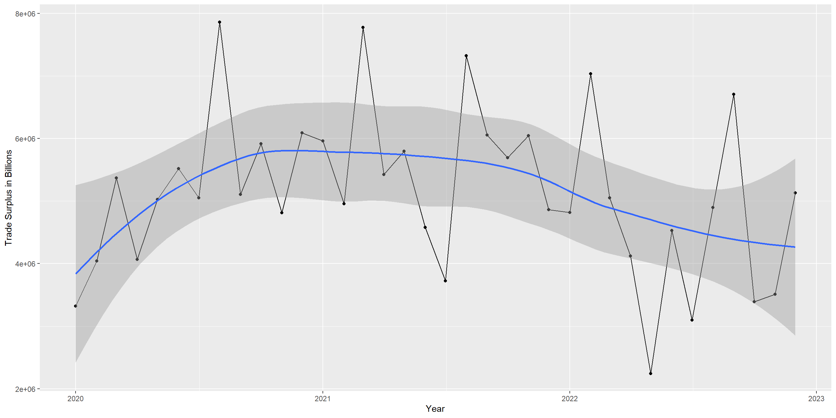
If we only look at the figure p1 above, one may say that Singapore trade data displayed a healthy uptrend both covid until recent 2022. However. once we examine the trade balance/surplus, Singapore trade surplus was only fluctuating between 3.5 billions and 8.5 billions on monthly basis and it is not on the steady uptrend at all.
Even at beginning of 2022, it even dropped to nearly 2.6 billions for Mar 2022 and that is the lowest level in 2 years period. If we look at the geom_smooth graph, we can see that the trade surplus of Singapore is actually on the downtrend since second half of 2020.
This contracts the general consensus that post-covid, with resume of commodities trades around the world, Singapore Trade surplus should be picking up. However, the data here suggests that as the world resumes normality, Singapore trade surplus is on the downtrend instead.
IMPORT VERSUS EXPORT - Monthly Cycle Plot
Next, based on the Trade Surplus above, we can create Monthly Cycle plot to compare the all the January between 2020 versus Jan in 2021, 2022 and 2023.
First, slice the the monthly_tradebalance into new data table with only 2 columns “Month-Year” and “Trade Surplus”
monthly_tradebalance_test = monthly_tradebalance[, c("Month-Year", "Trade_surplus")]
head(monthly_tradebalance_test)
Month-Year Trade_surplus
1 2020-01-01 3321432
2 2020-02-01 4039683
3 2020-03-01 5366990
4 2020-04-01 4067768
5 2020-05-01 5024021
6 2020-06-01 5519874Create 2 new columns in that data table, month and year from the Month-Year column
monthly_tradebalance_test <- monthly_tradebalance_test %>%
  mutate(year = year(monthly_tradebalance_test$`Month-Year`),
         month = factor(month(monthly_tradebalance_test$`Month-Year`), levels = 1:12,
                        labels = month.name))
We create horizontal lines with the Month that marked the average value of the trade surplus data.
monthly_tradebalance_test Month-Year Trade_surplus year month
1 2020-01-01 3321432 2020 January
2 2020-02-01 4039683 2020 February
3 2020-03-01 5366990 2020 March
4 2020-04-01 4067768 2020 April
5 2020-05-01 5024021 2020 May
6 2020-06-01 5519874 2020 June
7 2020-07-01 5049038 2020 July
8 2020-08-01 7861361 2020 August
9 2020-09-01 5106022 2020 September
10 2020-10-01 5914521 2020 October
11 2020-11-01 4814060 2020 November
12 2020-12-01 6092326 2020 December
13 2021-01-01 5960217 2021 January
14 2021-02-01 4958563 2021 February
15 2021-03-01 7775645 2021 March
16 2021-04-01 5422348 2021 April
17 2021-05-01 5795528 2021 May
18 2021-06-01 4579149 2021 June
19 2021-07-01 3726222 2021 July
20 2021-08-01 7324031 2021 August
21 2021-09-01 6053664 2021 September
22 2021-10-01 5694129 2021 October
23 2021-11-01 6045222 2021 November
24 2021-12-01 4864437 2021 December
25 2022-01-01 4818909 2022 January
26 2022-02-01 7033084 2022 February
27 2022-03-01 5052597 2022 March
28 2022-04-01 4121341 2022 April
29 2022-05-01 2243161 2022 May
30 2022-06-01 4527888 2022 June
31 2022-07-01 3095617 2022 July
32 2022-08-01 4897740 2022 August
33 2022-09-01 6707820 2022 September
34 2022-10-01 3393405 2022 October
35 2022-11-01 3508873 2022 November
36 2022-12-01 5130314 2022 Decemberavgvalue <- mean(monthly_tradebalance_test$Trade_surplus)
hline.data <- data.frame(avgvalue = avgvalue)ggplot(monthly_tradebalance_test, aes(x=year, y=Trade_surplus, group=month)) +
geom_line(colour="blue") +
geom_hline(aes(yintercept=avgvalue), data=hline.data, colour="blue", size=2) +
facet_grid(~month) +
xlab("Month of the Year") +
ylab("Trade Surplus in Billions") +
ggtitle("Singapore Trade Surplus Monthly Cycle Plot 2020 to 2023")+
scale_x_discrete(labels = function(x) substr(x, 3, 4))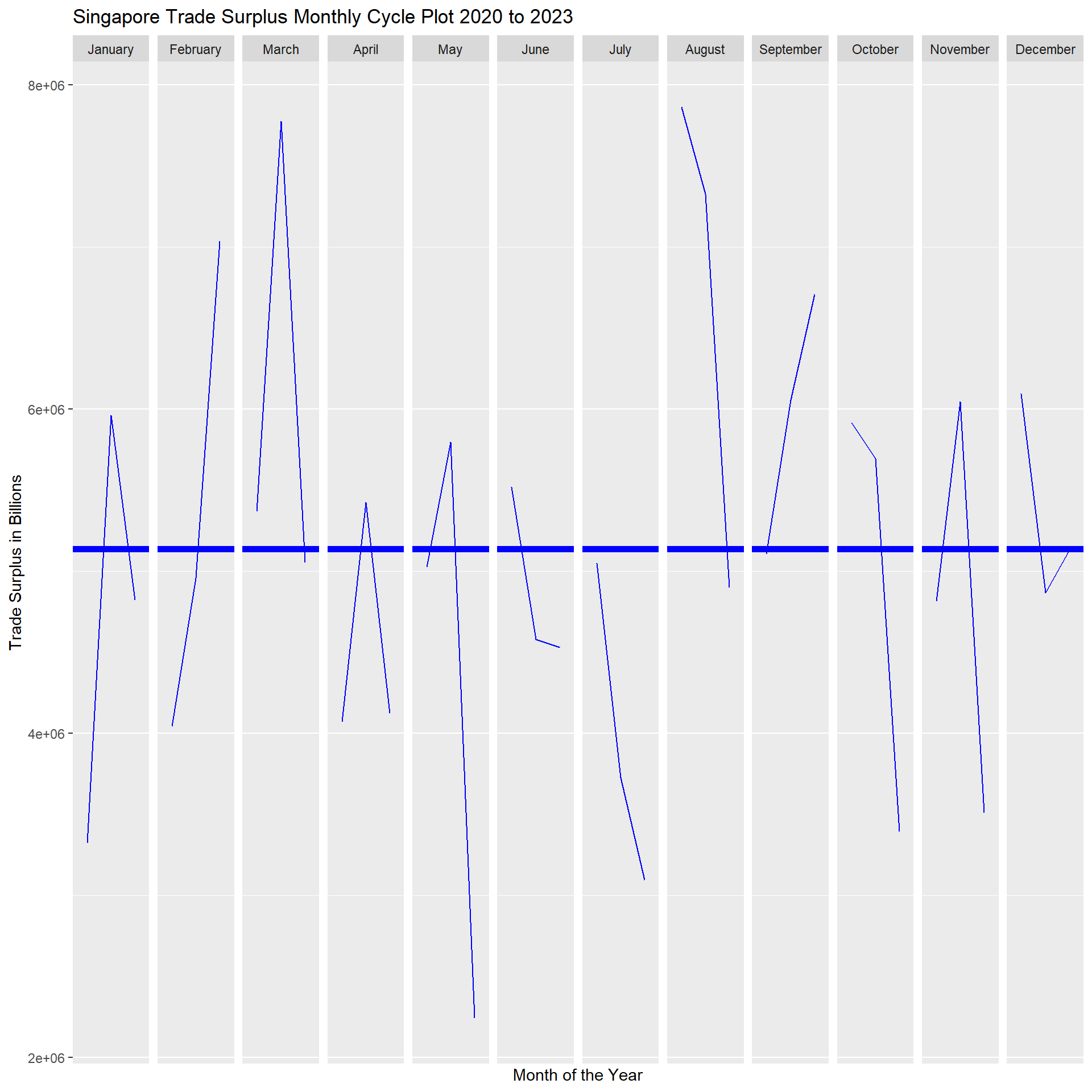
From above analysis, we can see that months with the highest trade surplus are March and August, where most of the trade surplus is above the monthly average of 5.1 billions. While April and July numbers were almost always below the average trade surplus.
Another observation is that almost across all the 12 months, the months of 2022 almost always is lower than the months of 2021 (except February) . In other words, Singapore trade surplus for 2022 are lower YoY basis, compared to 2021.
Contrary to prediction that Singapore trade balance will improve as Covid lockdowns around the world are lifted, as turbulent 2022 with record inflation and large scale war, Singapore trade surplus is actually not as good as previous 2021.
II) By Region
mthlyimport <- read_excel("C:/thomashoanghuy/ISSS608-VAA/TakehomeEx/data3/monthly data by countries.xlsx", sheet = "T1")

mthlyexport <- read_excel("C:/thomashoanghuy/ISSS608-VAA/TakehomeEx/data3/monthly data by countries.xlsx", sheet = "T2")
Let’s create a sub dataset for regions only, which consist of 6 areas, import and export
1) America
2) Asia
3) Europe
4) Oceania
5) Africa
Import Data
regions_mthlyimport = mthlyimport[1:6,]regions_mthlyexport = mthlyexport[1:6,]Combine 2 dataframes and transpose the data
regions_mthlytrade1 = rbind(regions_mthlyimport , regions_mthlyexport)
regions_mthlytrade= as.data.frame(t(regions_mthlytrade1))
colnames(regions_mthlytrade) <- regions_mthlytrade[1,]
regions_mthlytrade <- regions_mthlytrade[-1,]
regions_mthlytrade <- regions_mthlytrade %>%
rownames_to_column(var = "Month-Year")Reverse sort and convert the format of Month-Year to time and trade numbers into numeric format.
regions_mthlytrade <- regions_mthlytrade[nrow(regions_mthlytrade):1, ]
rownames(regions_mthlytrade) <- rownames(regions_mthlytrade[nrow(regions_mthlytrade):1, ])regions_mthlytrade$`Month-Year` <- as.Date(paste0(regions_mthlytrade$`Month-Year`, " 01"), format = "%Y %b %d")names(regions_mthlytrade)[2:7] <- c("Total Import", "America Import" , "Asia Import" , "Europe Import" , "Oceania Import", "Africa Import")names(regions_mthlytrade)[8:13] <- c("Total Export", "America Export" , "Asia Export" , "Europe Export" , "Oceania Export", "Africa Export")head(regions_mthlytrade) Month-Year Total Import America Import Asia Import Europe Import
1 2020-01-01 41180224.0 5844.1 27128.1 6859.7
2 2020-02-01 39472637.0 5314.1 26588.1 6209.6
3 2020-03-01 40433029.0 5910.8 26783.6 6333.3
4 2020-04-01 35878828.0 5183.5 24534.5 5150.6
5 2020-05-01 31458238.0 4259.0 21718.9 4629.0
6 2020-06-01 35120892.0 4686.2 24779.3 4960.7
Oceania Import Africa Import Total Export America Export Asia Export
1 819.7 528.6 44501656.0 5557.8 31668.0
2 694.7 666.1 43512320.0 5870.7 29713.9
3 845.9 559.4 45800019.0 6021.1 32534.9
4 637.6 372.6 39946596.0 6569.1 26245.7
5 441.8 409.6 36482259.0 5922.2 24437.8
6 456.4 238.2 40640766.0 4895.5 28994.5
Europe Export Oceania Export Africa Export
1 4432.5 2121.6 721.8
2 4996.4 2090.4 841.0
3 4468.2 1859.3 916.5
4 5051.3 1511.8 568.8
5 4398.0 1311.4 412.8
6 4880.4 1418.3 452.1Create dataframe for each region
america_data = regions_mthlytrade[, grepl("America", names(regions_mthlytrade))]
asia_data = regions_mthlytrade[, grepl("Asia", names(regions_mthlytrade))]
europe_data = regions_mthlytrade[, grepl("Europe", names(regions_mthlytrade))]
oceania_data = regions_mthlytrade[, grepl("Oceania", names(regions_mthlytrade))]
africa_data = regions_mthlytrade[, grepl("Africa", names(regions_mthlytrade))]
totalregion_data = regions_mthlytrade[, grepl("Total", names(regions_mthlytrade))]
america_data <- as.data.frame(lapply(america_data, function(x) as.numeric(as.character(x))))
asia_data <- as.data.frame(lapply(asia_data, function(x) as.numeric(as.character(x))))
europe_data <- as.data.frame(lapply(europe_data, function(x) as.numeric(as.character(x))))
oceania_data <- as.data.frame(lapply(oceania_data, function(x) as.numeric(as.character(x))))
africa_data <- as.data.frame(lapply(africa_data, function(x) as.numeric(as.character(x))))
totalregion_data <- as.data.frame(lapply(totalregion_data, function(x) as.numeric(as.character(x))))america_data$Month_Year <- regions_mthlytrade$`Month-Year`
asia_data$Month_Year <- regions_mthlytrade$`Month-Year`
europe_data$Month_Year <- regions_mthlytrade$`Month-Year`
oceania_data$Month_Year <- regions_mthlytrade$`Month-Year`
africa_data$Month_Year <- regions_mthlytrade$`Month-Year`
totalregion_data$Month_Year <- regions_mthlytrade$`Month-Year`AMERICA TRADE Volume
america_data <- america_data %>%
  mutate(fill = ifelse(America.Import > America.Export, "deficit", "surplus"))

americaplot = ggplot(america_data) +
  geom_line(aes(x = Month_Year, y = America.Import), stat = 'identity', color = "blue", size = 1) +
  geom_line(aes(x = Month_Year, y = America.Export), stat = 'identity', color = "darkred", size = 1) +
  geom_braid(aes(x = Month_Year, ymin = America.Import, ymax = America.Export, fill = fill), alpha = 0.5) +
  labs(x = "Year", y = "America Trade volume", title = "Americas Monthly Trade Balance") +
  scale_fill_manual(name = "Trade Balance",
                    values = c("deficit" = "brown" , "surplus" = "grey"))

americaplot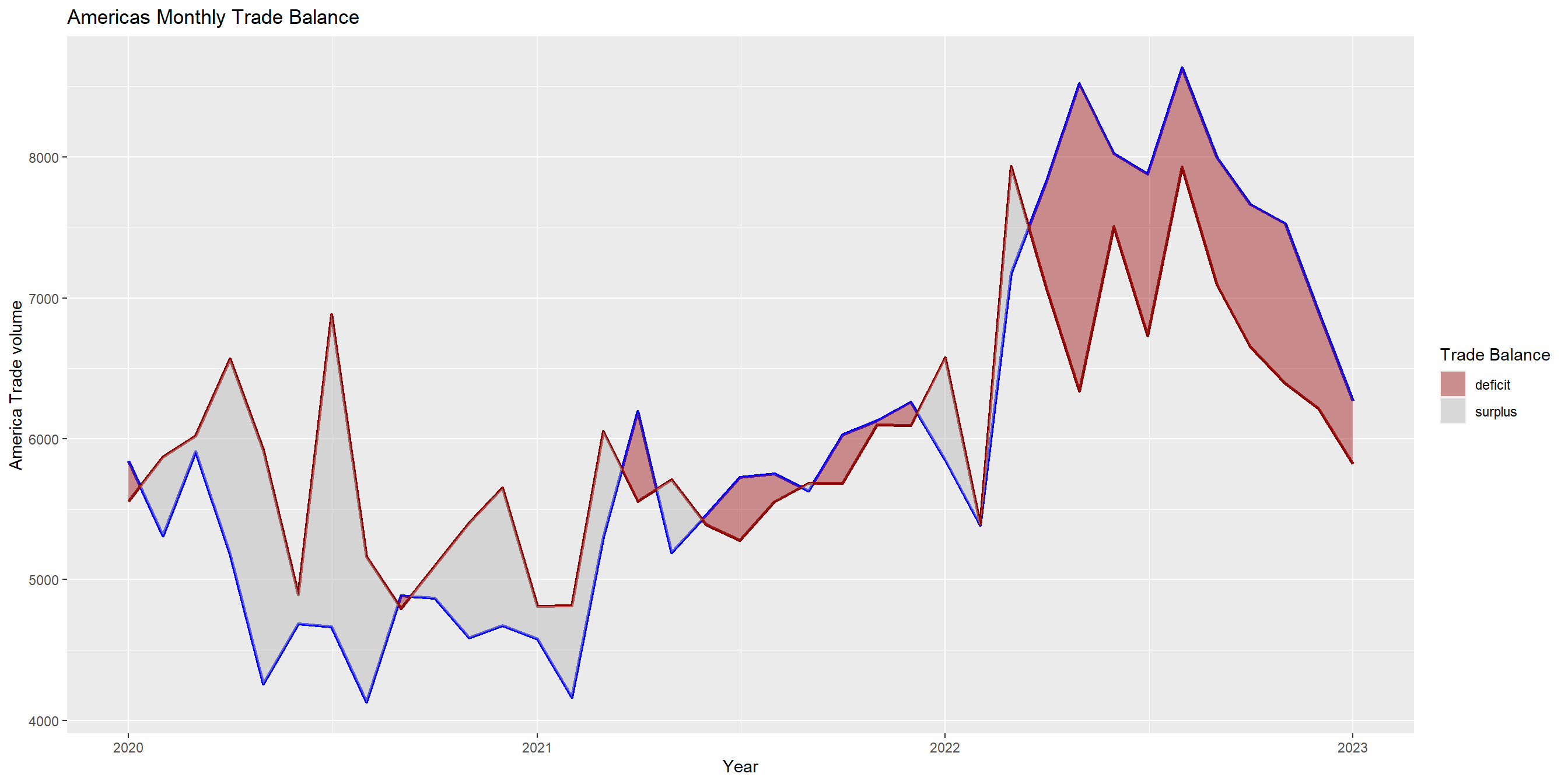
As you can see, the blue line represents the monthly Import number from America from Jan 2020 to Jan 2023. While dark red line represents the monthly Export number from America in the same period. With geom_braid color the difference area between the two lines in grey color, we can see the difference between the 2 lines clearly.
Throughout the time period, the Export figure was always above the blue line, which indicates Singapore was maintaining a trade surplus with Americas. However, as the grey area was getting smaller, proving Singapore trade surplus with America is getting smaller. And in 2021, the blue Import line started to cross above red Export line, this indicates Singapore import from America had exceeded export volume and Singapore started to enter into trade deficits versus Americas region.
This trade deficit has continued and even grew bigger in 2022, as evidenced by the bigger brown area between the 2 lines. This concludes that after Covid, Singapore from trade surplus position, has turned into deficit versus Americas regions
ASIA TRADE VOLUME
asia_data <- asia_data %>%
  mutate(fill = ifelse(Asia.Import > Asia.Export, "deficit", "surplus"))

asiaplot = ggplot(asia_data) +
  geom_line(aes(x = Month_Year, y = Asia.Import), stat = 'identity', color = "blue", size = 1) +
  geom_line(aes(x = Month_Year, y = Asia.Export), stat = 'identity', color = "darkred", size = 1) +
  geom_braid(aes(x = Month_Year, ymin = Asia.Import, ymax = Asia.Export, fill = fill), alpha = 0.5) +
  labs(x = "Year", y = "Asia Trade volume", title = "Asia Monthly Trade Balance") +
  scale_fill_manual(name = "Trade Balance",
                    values = c("deficit" = "brown" , "surplus" = "grey"))


asiaplot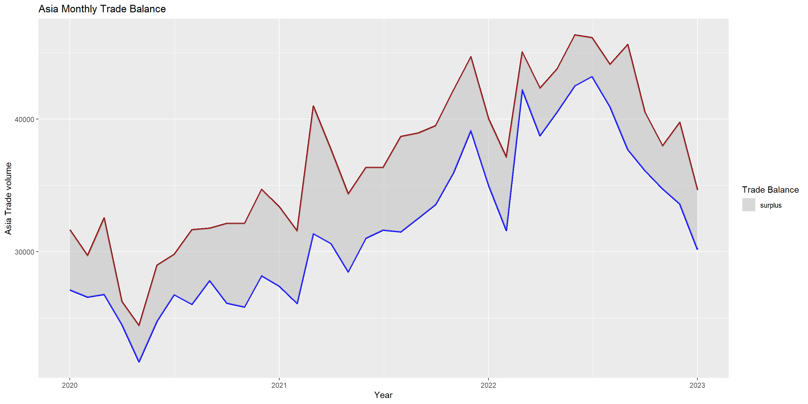
EUROPE TRADE VOLUME
europe_data <- europe_data %>%
  mutate(fill = ifelse(Europe.Import > Europe.Export, "deficit", "surplus"))

europeplot = ggplot(europe_data) +
  geom_line(aes(x = Month_Year, y = Europe.Import), stat = 'identity', color = "blue", size = 1) +
  geom_line(aes(x = Month_Year, y = Europe.Export), stat = 'identity', color = "darkred", size = 1) +
  geom_braid(aes(x = Month_Year, ymin = Europe.Import, ymax = Europe.Export, fill = fill), alpha = 0.5) +
  labs(x = "Year", y = "Europe Trade volume", title = "Europe Monthly Trade Balance") +
  scale_fill_manual(name = "Trade Balance",
                    values = c("deficit" = "brown" , "surplus" = "grey"))


europeplot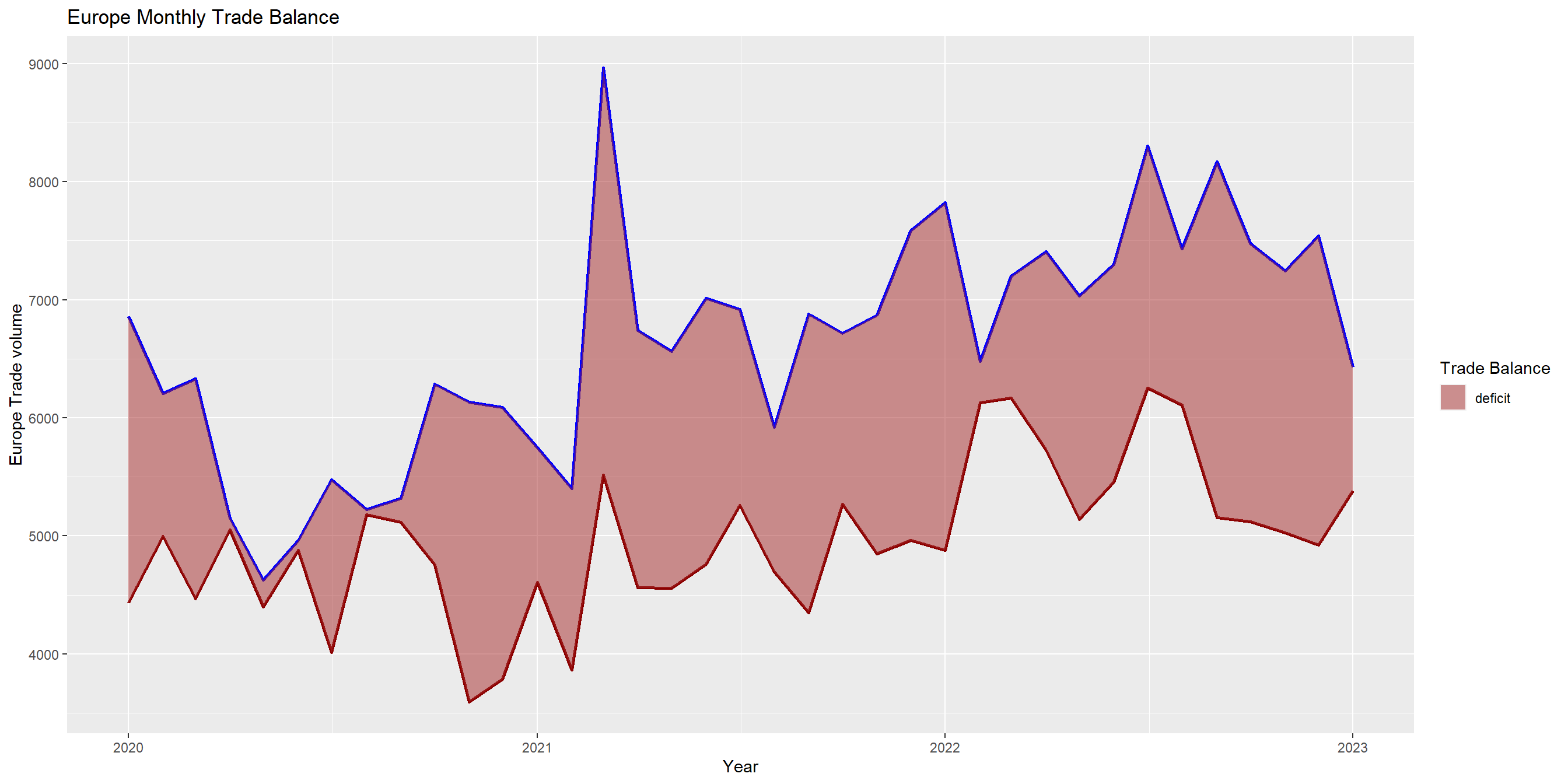
OCEANIA TRADE VOLUME
oceania_data <- oceania_data %>%
  mutate(fill = ifelse(Oceania.Import > Oceania.Export, "deficit", "surplus"))

oceaniaplot = ggplot(oceania_data) +
  geom_line(aes(x = Month_Year, y = Oceania.Import), stat = 'identity', color = "blue", size = 1) +
  geom_line(aes(x = Month_Year, y = Oceania.Export), stat = 'identity', color = "darkred", size = 1) +
  geom_braid(aes(x = Month_Year, ymin = Oceania.Import, ymax = Oceania.Export, fill = fill), alpha = 0.5) +
  labs(x = "Year", y = "Oceania Trade volume", title = "Oceania Monthly Trade Balance") +
  scale_fill_manual(name = "Trade Balance",
                    values = c("deficit" = "brown" , "surplus" = "grey"))

oceaniaplot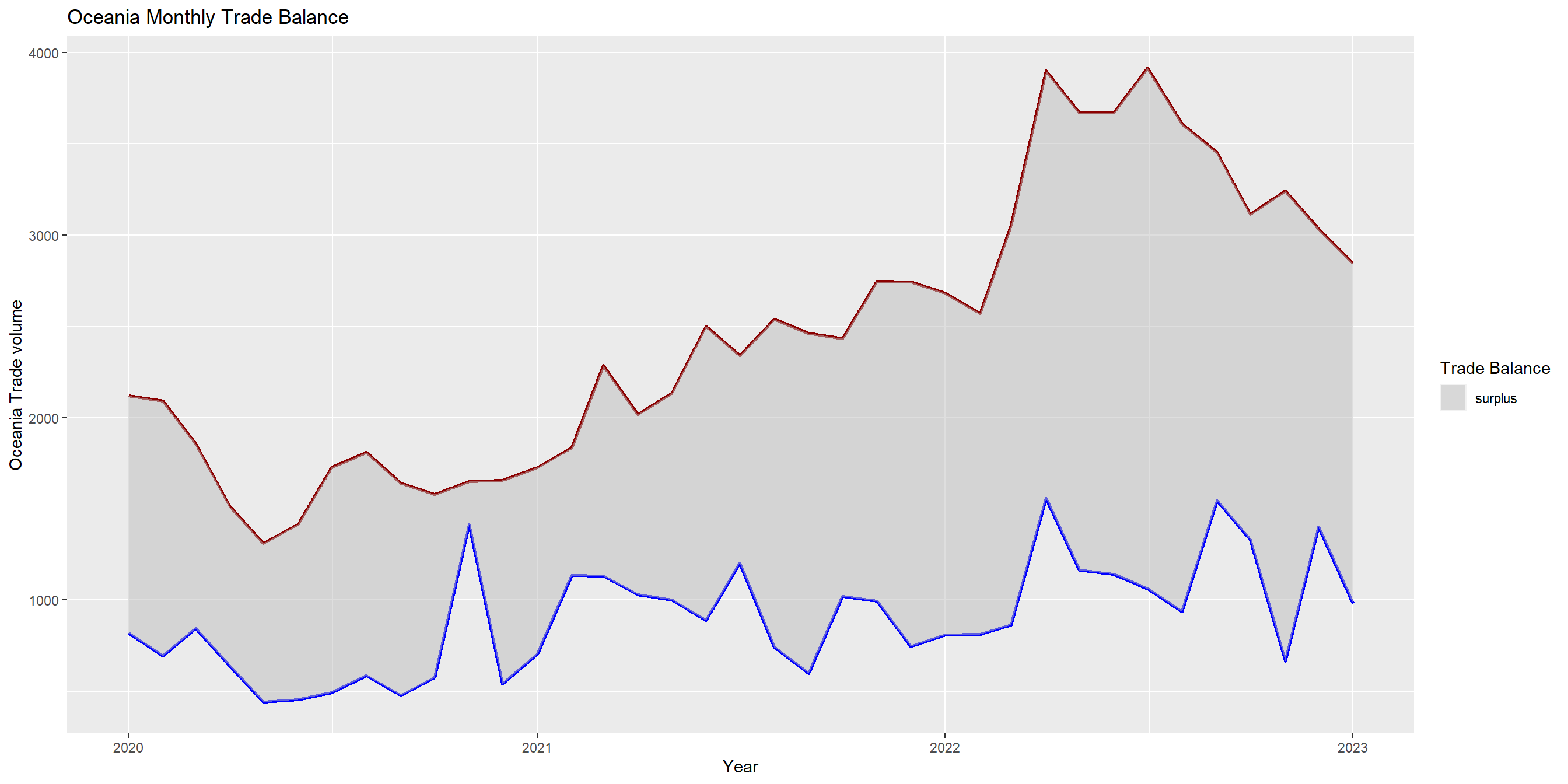
AFRICA TRADE VOLUME
africa_data <- africa_data %>%
  mutate(fill = ifelse(Africa.Import > Africa.Export, "deficit", "surplus"))

africaplot = ggplot(africa_data) +
  geom_line(aes(x = Month_Year, y = Africa.Import), stat = 'identity', color = "blue", size = 1) +
  geom_line(aes(x = Month_Year, y = Africa.Export), stat = 'identity', color = "darkred", size = 1) +
  geom_braid(aes(x = Month_Year, ymin = Africa.Import, ymax = Africa.Export, fill = fill), alpha = 0.5) +
  labs(x = "Year", y = "Africa Trade volume", title = "Africa Monthly Trade Balance") +
  scale_fill_manual(name = "Trade Balance",
                    values = c("deficit" = "brown" , "surplus" = "grey"))

africaplot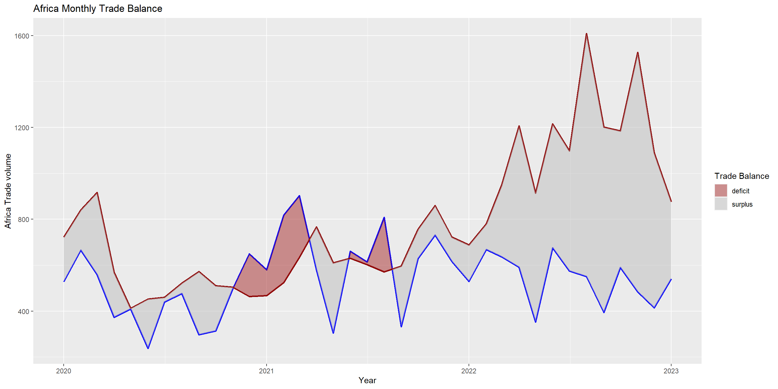
OVERALL TRADE VOLUME
totalregion_data <- totalregion_data %>%
  mutate(fill = ifelse(Total.Import > Total.Export, "deficit", "surplus"))

overallplot = ggplot(totalregion_data) +
  geom_line(aes(x = Month_Year, y = Total.Import), stat = 'identity', color = "blue", size = 1) +
  geom_line(aes(x = Month_Year, y = Total.Export), stat = 'identity', color = "darkred", size = 1) +
  geom_braid(aes(x = Month_Year, ymin = Total.Import, ymax = Total.Export, fill = fill), alpha = 0.5) +
  labs(x = "Year", y = "Overall Trade volume", title = "Overall Monthly Trade Balance") +
  scale_fill_manual(name = "Trade Balance",
                    values = c("deficit" = "brown" , "surplus" = "grey"))

overallplot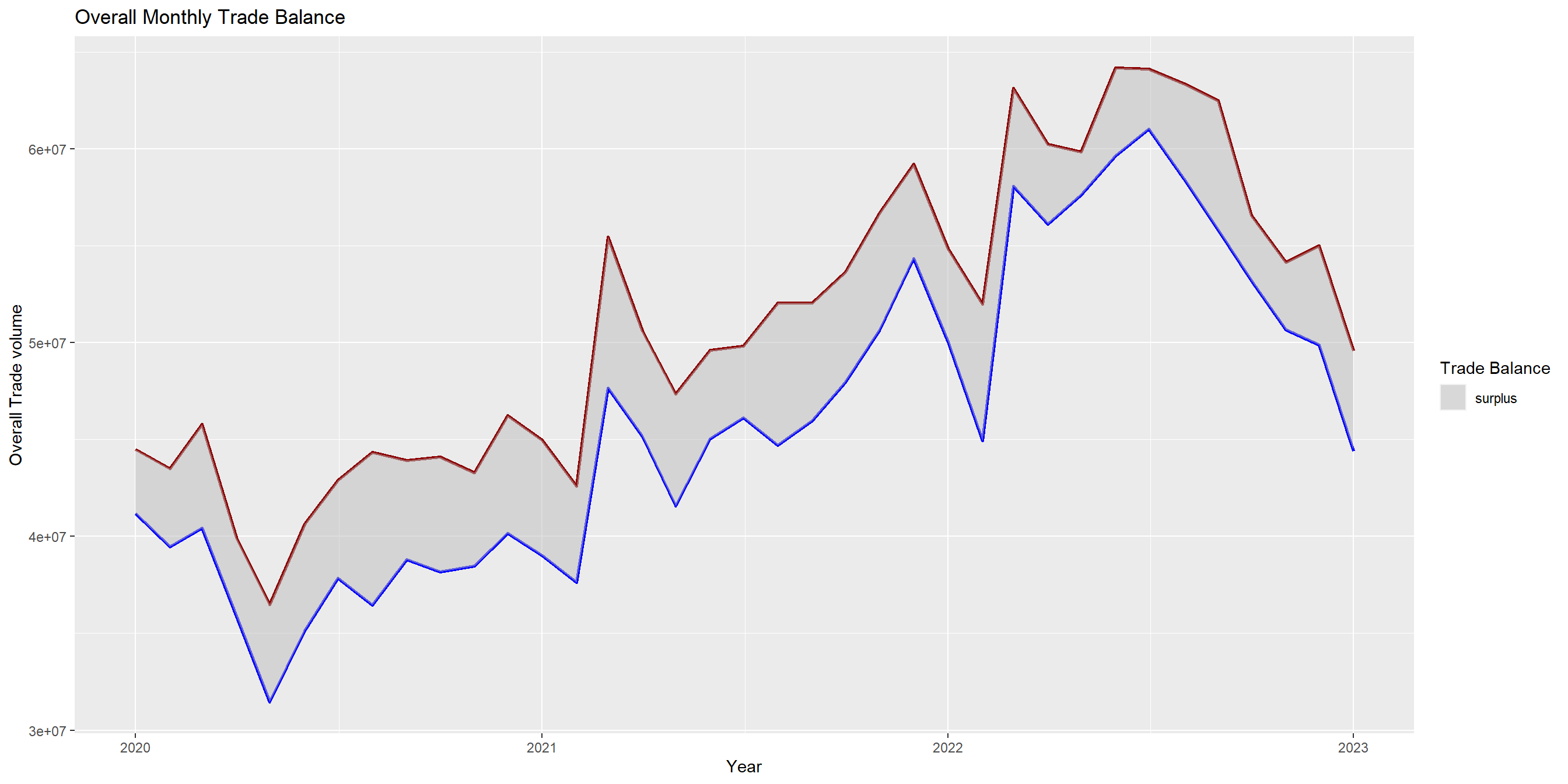
Dashboard for Regions Data
(americaplot + asiaplot + europeplot) / (oceaniaplot + africaplot + overallplot)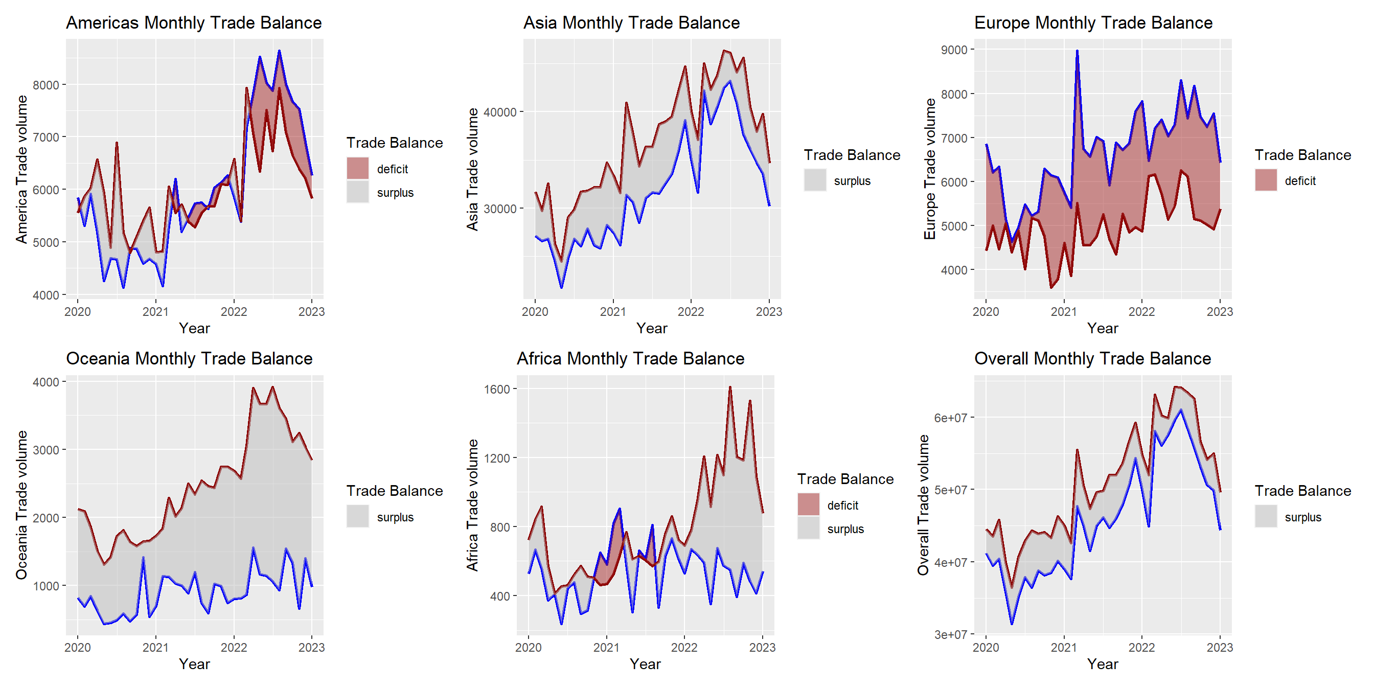
In this dashboard, we can compare Singapore monthly trade blances (surplus / deficits) versus 5 main regions of world geography. In term of volume, Asia trade balance is the highest, with both import and export numbers reaching to the height of more than 40 billions per month, while Oceania trade number is the lowest reaching no more than 4 billions SGD monthly. The grey area represents the periods where Singapore is enjoying trade surplus against its trading partners, while the brown area is where Singapore dipped into trade deficit monthly.
In term of trend, Americas portrayed a reverse between 2020 to 2022, where during Covid lockdown, Singapore was holding trade surplus with Americas, but once lockdown was lifted, Singapore has turned into trade deficit versus Americas.
In Oceania, and Africa, Singapore has been maintaining positive trade surplus, regardless of the covid lockdown. The noticeable difference is the grey area (represents the trade surplus if the red line is above the blue line) is getting bigger in 2022, compared to previous years
In Europe, Singapore has always been having trade deficit (blue line is above the red line), and the deficit (brown area) seems to get bigger from 2020 to 2022, too as the covid lockdown started to lift. One would expect that due to Russian invasion, which disrupted the transportation and production of goods and services in Europe, Singapore as an import partner, would have its import decrease and smaller trade deficit. But apparently, the trade deficit gets even larger as per this evidence.
Overall plot, we can see that it mimics the trend of 2 biggest trading regional partners with Singapore, Asia and Americas, where the export and import volumes were trending up until mid year 2022, and they both started to trend downward. This can be the impact of Russian invasion on Ukraine, combined with huge inflation and tightening of money supplies by most superpowers around the world, lead to the dampening of trade volume.
Both the import and export volumes have pickup tremendeously from 2020 to 2022. However, Americas and Asia graphs above have shown, the second half of 2022 have seen an reverse in the uptrend of trade volumes, signalling that there may be a cool-down in the trade activities, and possibly an negative indicator for economic growth.
What about other countries?
Using the above code chunks, we can examine other countries, which are major trading partners with Singapore. Let’s check out some of them.
China
Import Data
china_mthlyimport = mthlyimport[grep("China", mthlyimport$`Data Series`, ignore.case = TRUE), ]china_mthlyexport = mthlyexport[grep("China", mthlyexport$`Data Series`, ignore.case = TRUE), ]Combine 2 dataframes and transpose the data
china_mthlytrade1 = rbind(china_mthlyimport , china_mthlyexport)
china_mthlytrade= as.data.frame(t(china_mthlytrade1))
colnames(china_mthlytrade) <- china_mthlytrade[1,]
china_mthlytrade <- china_mthlytrade[-1,]
china_mthlytrade <- china_mthlytrade %>%
rownames_to_column(var = "Month-Year")Reverse sort and convert the format of Month-Year to time and trade numbers into numeric format.
china_mthlytrade <- china_mthlytrade[nrow(china_mthlytrade):1, ]
rownames(china_mthlytrade) <- rownames(china_mthlytrade[nrow(china_mthlytrade):1, ])china_mthlytrade$`Month-Year` <- as.Date(paste0(china_mthlytrade$`Month-Year`, " 01"), format = "%Y %b %d")
names(china_mthlytrade)[2:3] <- c("China Import", "China Export")china_mthlytrade$`China Import` = as.numeric(china_mthlytrade$`China Import`)
china_mthlytrade$`China Export` = as.numeric(china_mthlytrade$`China Export`)Now we can plot our data
china_mthlytrade <- china_mthlytrade %>%
  mutate(fill = ifelse( china_mthlytrade$`China Import`> china_mthlytrade$`China Export`, "deficit", "surplus"))

chinaplot = ggplot(china_mthlytrade) +
  geom_line(aes(x = china_mthlytrade$`Month-Year`, y = china_mthlytrade$`China Import`), stat = 'identity', color = "blue", size = 1) +
  geom_line(aes(x = china_mthlytrade$`Month-Year`, y = china_mthlytrade$`China Export`), stat = 'identity', color = "darkred", size = 1) +
  geom_braid(aes(x = china_mthlytrade$`Month-Year`, ymin = china_mthlytrade$`China Export`, ymax = china_mthlytrade$`China Import`, fill = fill), alpha = 0.5) +
  labs(x = "Year", y = "China Trade volume", title = "China Monthly Trade Balance" ) +
  scale_fill_manual(name = "Trade Balance",
                    values = c("deficit" = "brown" , "surplus" = "grey"))

chinaplot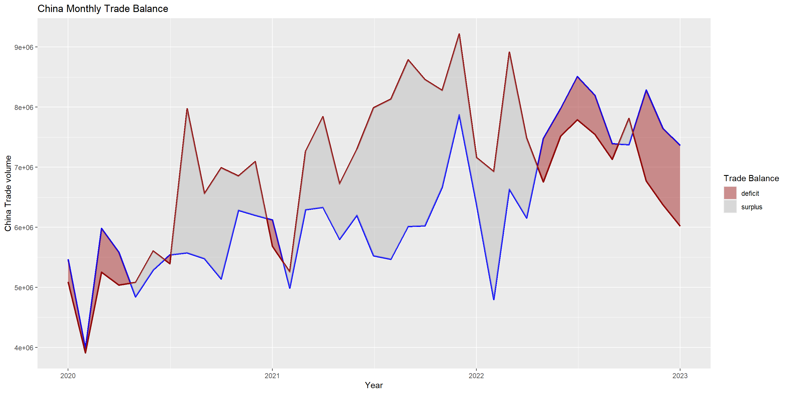
China is one of the Singapore’s largest trade partner. As you can see from the above charts, both Singapore import and export volumes with China have increased from 2020 to 2023. The numbers have more than doubled from 4 billions to 9 billions. The dark red line represented the Export, while blue line represents the monthly import. A
At beginning of 2020, the brown area by geom_braid suggested that Singapore has a small trade deficit with China. However from April 2020 all to April 2022, we can see that the red line always stayed above the blue line, which suggest Singapore was maintaining the trade surplus ( which is represented by the grey area). Understandably, this is due to China pursued the zero Covid policy which severely affected their manufacturing capabilities and thus Singapore cannot import from China as much.
As the Russian invasion happened mid-2022 and covid lockdown lifted by Singapore, the trade balance has turned deficit again, by sharp decrease of Singapore export to China.
However, trade deficit may not be a bad case in this scenario, the reason is SGD is stronger than Chinese yuan. In a trade deficit environment, that allows Singapore to import more goods and service from China at lower cost ( cuz 1 SGD can purchase more of Chinese goods) and ultimately benefit the consumers in Singapore.
Malaysia
Let’s reuse the same code sample and apply on other countries.
Malaysia_mthlyimport = mthlyimport[grep("Malaysia", mthlyimport$`Data Series`, ignore.case = TRUE), ]Malaysia_mthlyexport = mthlyexport[grep("Malaysia", mthlyexport$`Data Series`, ignore.case = TRUE), ]Combine 2 dataframes and transpose the data
Malaysia_mthlytrade1 = rbind(Malaysia_mthlyimport , Malaysia_mthlyexport)
Malaysia_mthlytrade= as.data.frame(t(Malaysia_mthlytrade1))
colnames(Malaysia_mthlytrade) <- Malaysia_mthlytrade[1,]
Malaysia_mthlytrade <- Malaysia_mthlytrade[-1,]
Malaysia_mthlytrade <- Malaysia_mthlytrade %>%
rownames_to_column(var = "Month-Year")Reverse sort and convert the format of Month-Year to time and trade numbers into numeric format.
Malaysia_mthlytrade <- Malaysia_mthlytrade[nrow(Malaysia_mthlytrade):1, ]
rownames(Malaysia_mthlytrade) <- rownames(Malaysia_mthlytrade[nrow(Malaysia_mthlytrade):1, ])Malaysia_mthlytrade$`Month-Year` <- as.Date(paste0(Malaysia_mthlytrade$`Month-Year`, " 01"), format = "%Y %b %d")
names(Malaysia_mthlytrade)[2:3] <- c("Malaysia Import", "Malaysia Export")Malaysia_mthlytrade$`Malaysia Import` = as.numeric(Malaysia_mthlytrade$`Malaysia Import`)
Malaysia_mthlytrade$`Malaysia Export` = as.numeric(Malaysia_mthlytrade$`Malaysia Export`)Now we can plot our data
tail(Malaysia_mthlytrade) Month-Year Malaysia Import Malaysia Export
32 2022-08-01 7225607 6150507
33 2022-09-01 7672003 5884698
34 2022-10-01 6417377 6233818
35 2022-11-01 6773423 5557119
36 2022-12-01 6017970 5154779
37 2023-01-01 4840965 4987116Malaysia_mthlytrade <- Malaysia_mthlytrade %>%
mutate(fill = ifelse( Malaysia_mthlytrade$`Malaysia Import`> Malaysia_mthlytrade$`Malaysia Export`, "deficit", "surplus"))
Malaysiaplot = ggplot(Malaysia_mthlytrade) +
geom_line(aes(x = Malaysia_mthlytrade$`Month-Year`, y = Malaysia_mthlytrade$`Malaysia Import`), stat = 'identity', color = "blue", size = 1) +
geom_line(aes(x = Malaysia_mthlytrade$`Month-Year`, y = Malaysia_mthlytrade$`Malaysia Export`), stat = 'identity', color = "darkred", size = 1) +
geom_braid(aes(x = Malaysia_mthlytrade$`Month-Year`, ymin = Malaysia_mthlytrade$`Malaysia Export`, ymax = Malaysia_mthlytrade$`Malaysia Import`, fill = fill), alpha = 0.5) +
labs(x = "Year", y = "Malaysia Trade volume", title = "Malaysia Monthly Trade Balance" ) +
scale_fill_manual(name = "Trade Balance",
values = c("deficit" = "brown" , "surplus" = "grey"))
Malaysiaplot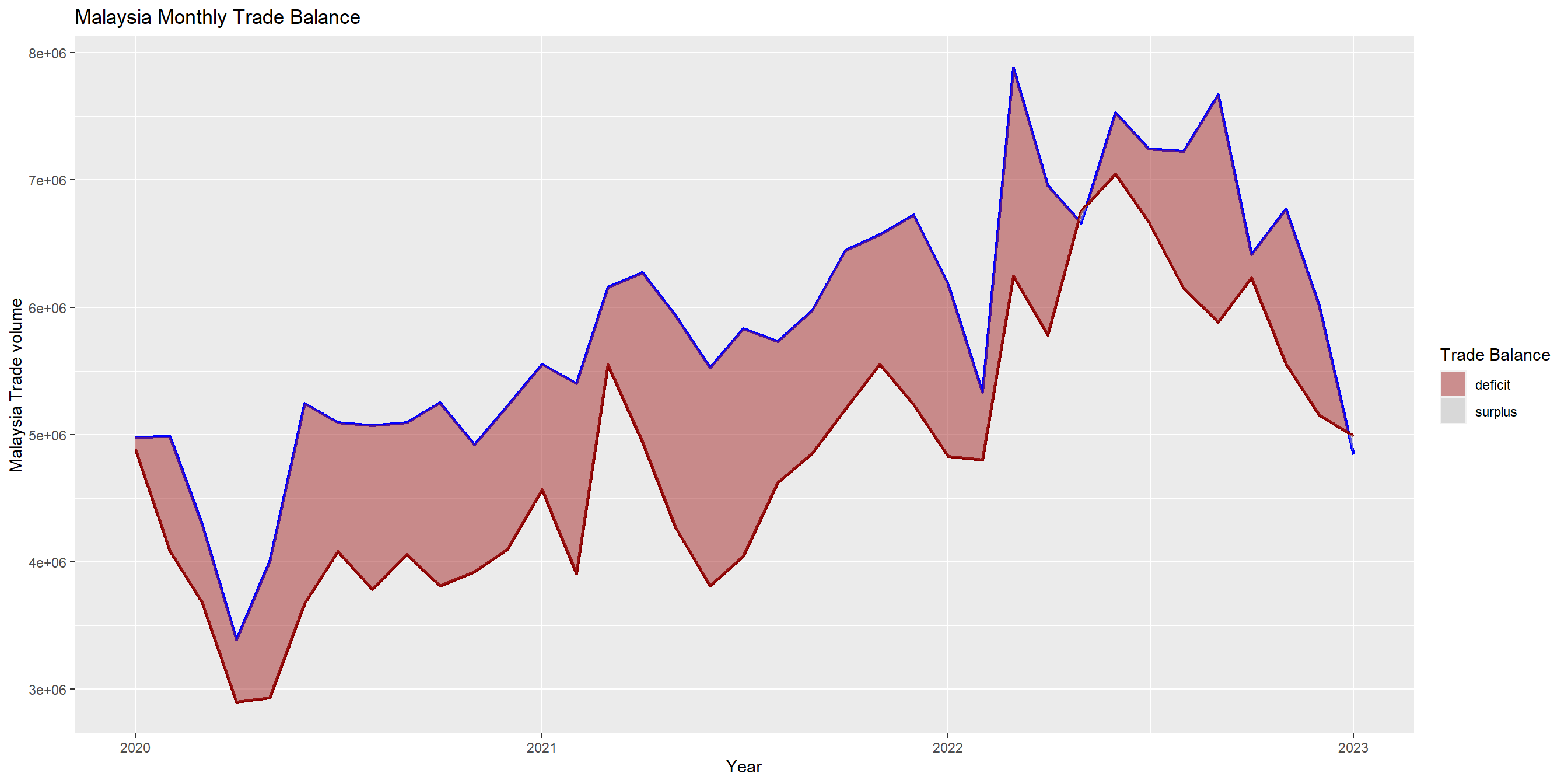
For Malaysia, Singapore has always been maintaining a trade deficit with northern neighbour Malaysia throughout 2020 to 2023. However as the 2023 coming, the brown area (represents the trade deficit) has been getting smaller, proving that there could be a change in near future. Singapore may actually become net export partner to Malaysia.
Similar to China above, a SGD is stronger than Malaysian ringgit, which allows 1 SGD to purchase more of Malaysian imported goods and services, this may benefit Singapore consumers and boost Singapore economy. So it is understandable that Singapore government wants to maintain trade deficit with Malaysia.
Both the import and export volumes have pickup tremendeously from 2020 to 2022. However similar to Americas and Asia graphs above, the second half of 2022 have seen an reverse in the uptrend of trade volumes, signalling that there may be a cooldown in the trade activities, and possibly an negative indicator for economic growth.
Vietnam
Vietnam_mthlyimport = mthlyimport[grep("Vietnam", mthlyimport$`Data Series`, ignore.case = TRUE), ]Vietnam_mthlyexport = mthlyexport[grep("Vietnam", mthlyexport$`Data Series`, ignore.case = TRUE), ]Combine 2 dataframes and transpose the data
Vietnam_mthlytrade1 = rbind(Vietnam_mthlyimport , Vietnam_mthlyexport)
Vietnam_mthlytrade= as.data.frame(t(Vietnam_mthlytrade1))
colnames(Vietnam_mthlytrade) <- Vietnam_mthlytrade[1,]
Vietnam_mthlytrade <- Vietnam_mthlytrade[-1,]
Vietnam_mthlytrade <- Vietnam_mthlytrade %>%
rownames_to_column(var = "Month-Year")Reverse sort and convert the format of Month-Year to time and trade numbers into numeric format.
Vietnam_mthlytrade <- Vietnam_mthlytrade[nrow(Vietnam_mthlytrade):1, ]
rownames(Vietnam_mthlytrade) <- rownames(Vietnam_mthlytrade[nrow(Vietnam_mthlytrade):1, ])Vietnam_mthlytrade$`Month-Year` <- as.Date(paste0(Vietnam_mthlytrade$`Month-Year`, " 01"), format = "%Y %b %d")
names(Vietnam_mthlytrade)[2:3] <- c("Vietnam Import", "Vietnam Export")Vietnam_mthlytrade$`Vietnam Import` = as.numeric(Vietnam_mthlytrade$`Vietnam Import`)
Vietnam_mthlytrade$`Vietnam Export` = as.numeric(Vietnam_mthlytrade$`Vietnam Export`)Now we can plot our data
Vietnam_mthlytrade <- Vietnam_mthlytrade %>%
  mutate(fill = ifelse( Vietnam_mthlytrade$`Vietnam Import`> Vietnam_mthlytrade$`Vietnam Export`, "deficit", "surplus"))

Vietnamplot = ggplot(Vietnam_mthlytrade) +
  geom_line(aes(x = Vietnam_mthlytrade$`Month-Year`, y = Vietnam_mthlytrade$`Vietnam Import`), stat = 'identity', color = "blue", size = 1) +
  geom_line(aes(x = Vietnam_mthlytrade$`Month-Year`, y = Vietnam_mthlytrade$`Vietnam Export`), stat = 'identity', color = "darkred", size = 1) +
  geom_braid(aes(x = Vietnam_mthlytrade$`Month-Year`, ymin = Vietnam_mthlytrade$`Vietnam Export`, ymax = Vietnam_mthlytrade$`Vietnam Import`, fill = fill), alpha = 0.5) +
  labs(x = "Year", y = "Vietnam Trade volume", title = "Vietnam Monthly Trade Balance" ) +
  scale_fill_manual(name = "Trade Balance",
                    values = c("deficit" = "brown" , "surplus" = "grey"))

Vietnamplot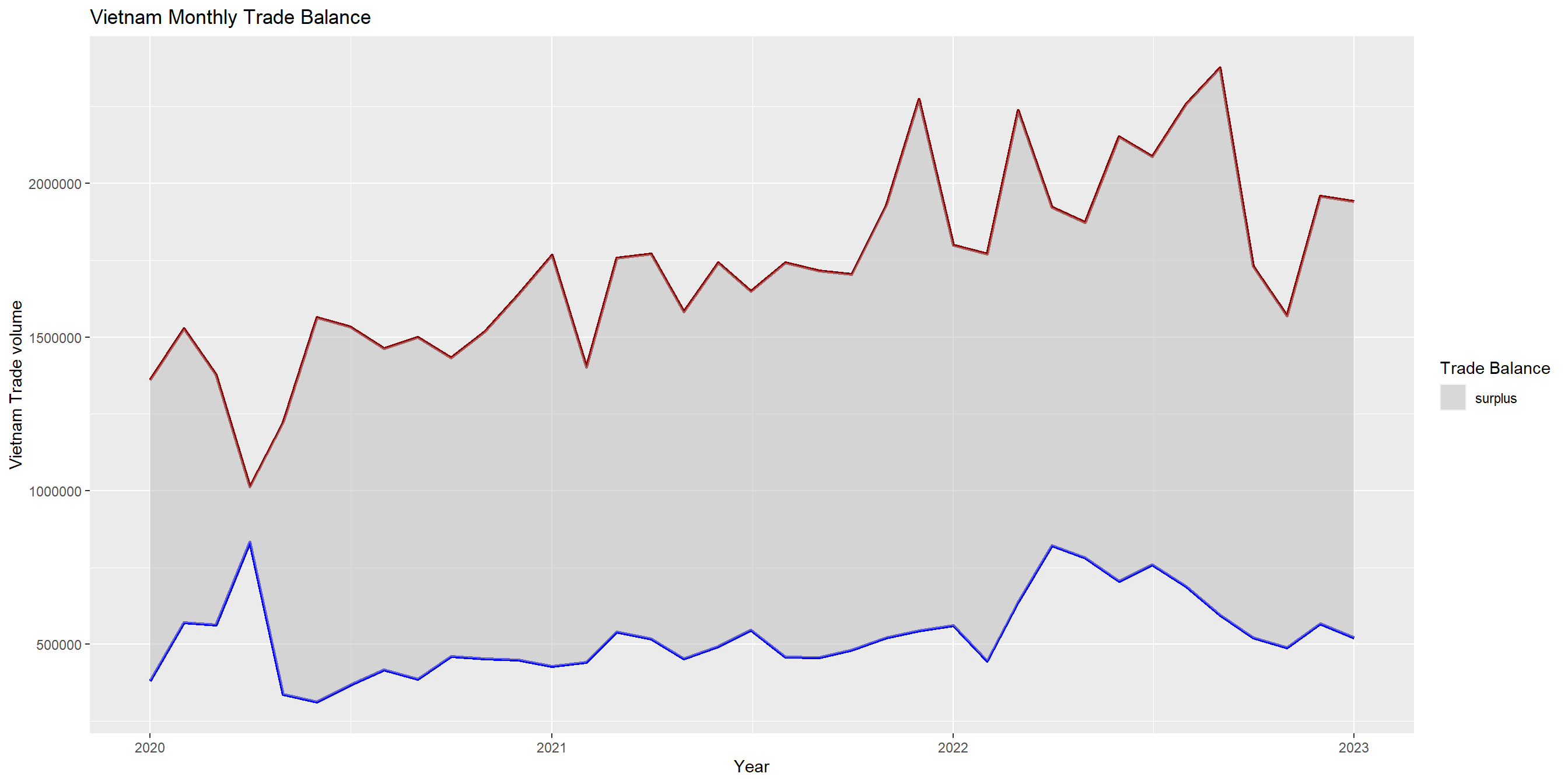
Vietnam is one of the huge agricultural export country in the South East Asia region, it’s popular belief that a lot of finished consumer goods, and agricultural products in Singapore is imported from Vietnam, however the above graph depicts that Singapore is actually a net-export country to Vietnam where the trade surplus versus Vietnam is huge. Throughout covid, 2020 to 2022, the import of Singapore from Vietnam is actually relatively stable, proving that covid 19 did not affect Vietnam manufacturing of exports to Singapore.
But with 1 SGD = 17,000 VND (as SGD is much stronger currency), this also means Singapore average consumers are paying higher prices for Vietnamese goods and services, and this may intensify the effect of inflation on Singapore population. This is actually not good, considering Singapore inflation is hitting record high in 2022.
Conclusion
The above analyses have given a few representation of Singapore trade activities post covid pandemic, which have been quite challenging on economies and all countries. Overall, immediately after 2019, Singapore has seen a steady recovery and uptrend in both import and export trade volumes. While Singapore wants to leverage upon her strong SGD and maintain status quo of trade balance versus her trading partners, however there are some reversal in the case of Americas and China.
Ultimately, this also shows that while Covid pandemics may be behind Singapore, Singapore economy is still facing a huge head-winds ahead, facing with uncertainties from global wars, conflicts with superpower and the impending effect of high inflation that directly affected the average consumers in Singapore.
Self-Relfection
This is a great and very challenging exercise, that teaches me how to deal with Time-series data. In term of Data wrangling, I learnt different ways to manipulate tables, to slice and subset as well as transform the data to fit the suitable formats to be used to plot graph.
Moreover, I have learned and put into practice how to draw graphs such as Cycle Plot, the Geom_braid as well as I also learned we can design and use each geom functions as its own graphs before combining them under ggplot.
I have also learned to combine multiple plots into trellis style dashboard, something I was not able to do a few week earlier.
Area of improvement: still data wrangling. I believe that there are better ways to manipulate data tables, leveraging on mutate() and group_by() function.
I think the best way to learn is backward reverse engineering when I can see / imagine the result desired dataframe (which will be fed into ggplot) and compare them versus the raw data table and figure which methods / functions that can allow me to transform from raw data table to desired datasets.